Where Graph Theory Meets The Road: The Algorithms Behind Route Planning [Hackaday]

View Article on Hackaday

Back in the hazy olden days of the pre-2000s, navigating between two locations generally required someone to whip out a paper map and painstakingly figure out the most optimal route between those depending on the chosen methods of transport. For today’s generations no such contrivances are required, with technology having obliterated even the a need to splurge good money on a GPS navigation device and annual map updates.

These days, you get out a computing device, open Google Maps or equivalent, ask it how you should travel somewhere, and most of the time the provided route will be the correct one, including the fine details such as train platform and departure times. Yet how does all of this seemingly magical route planning technology work? It’s often assumed that Dijkstra’s algorithm, or the A* graph traversal algorithm is used, but the reality is that although these pure graph theory algorithms are decidedly influential, they cannot be applied verbatim to the reality of graph traversal between destinations in the physical world.

A Story Of Travelers

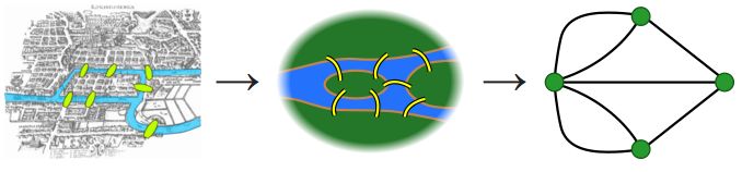
The field of graph theory has been around since 1736, when Leonhard Euler published an article on the subject of the Seven Bridges of Königsberg (in Prussia, today’s Kaliningrad in Russia). In this mathematical problem a walk has to be devised through the city in which each of the seven bridges across the city’s Pregel River that connect to the two islands in said river is only crossed once. Euler observed that the only relevant information here are the land masses (the nodes) and the connections between them (the bridges, or edges), which reduces the problem to a simple graph.

On this graph a starting node is selected, with another node as the end node. As each land mass is connected with an odd number of bridges (3 or 5), this means that this problem does not have a solution. The main challenge here lies in devising a mathematically acceptable proof of this impossibility, which is where the foundations for what we today know as graph theory.

From here graph theory got expanded and generalized into relations between objects, finding use in fields from computer science and chemistry to biology and linguistics. Combined with algorithms that can handle such graphs it’s a great way to not only make the basic structure of a network clear, but also to model structures and systems. Naturally, finding a route between nodes remained a crucial part of the field, with a wide range of path finding algorithms developed over the centuries.

Perhaps the most common graph theory problem is that of the Travelling Salesman Problem (TSP), which is somewhat like Euler’s original seven bridge problem, but instead asks for a traveller (a salesman) to be guided between a collection of cities in the most efficient way possible. The trick here is that by blindly trying out each route, the number of possible routes increases rapidly with each added city. By modeling the cities as nodes, an algorithm can then be devised that creates the edges between nodes, taking into account the weight of each node, related to its position on the map.

Although simple route planning is not as daunting as TSP, there are some similarities, in that it involves a weighted, undirected graph, requiring the algorithm to take into account the cost of each edge as well as the total cost, creating a minimum spanning tree. One of the first algorithms for this is Jarník’s algorithm, by Czech mathematician Vojtěch Jarník in 1930. Later this was rediscovered by Robert C. Prim in 1957 and in 1956 by Edsger W. Dijkstra (Dijkstra’s algorithm).

The weight assigned to each node is the Euclidian distance, allowing the the algorithm to calculate the distance of any newly discovered node to its current node. In its most simple form as a path finding algorithm, it tries one or more steps in roughly the direction of the destination and selects the shortest branch from these, repeating this procedure until the destination has been reached and something close to the shortest path has been found.

The most well-known improvement to this basic algorithm is probably the A* algorithm (geometric goal directed search), which was developed in 1968 at Stanford Research Institute. Rather than a simple node-to-node algorithm, A* considers the entirety of the nodes, and may skip nearby nodes in order to achieve an overall shorter path between the source and destination. One disadvantage of A* is that it has to keep all nodes in memory, making it much more memory-intensive than alternatives. Despite this, A* has been the usual choice for path finding in the real world.

GPS For Everyone

Before the US enabled higher accuracy with the GPS satellites by turning off Selective Availability (SA), the best precision you could hope for by default was about 50-100 meters. This was clearly not enough to use for live navigation which – along with the high prices for satellite navigation devices during the 1990s – left route planning mostly dependent on paper maps and scribbled-down notes along with the occasional updates from helpful locals. Route planning using automated means was already used at this time, but the biggest use was by route planners at railways, logistics companies and so on.

With highly accurate GPS positioning becoming available in 2000 without the need for SA correction algorithms, and later other global navigation satellite systems (GNSS) becoming available to the public alongside rapidly dropping prices for GNSS-enabled devices, suddenly it became possible to combine digital maps with accurate satellite navigation, far beyond the scope of early satnav devices during the 1990s. This would lead eventually to the rise of smartphones, with their wireless internet connectivity, built-in GNSS support and apps like Google Maps that quite literally put a satnav device into your pocket.

Although it’s useful to get live updates from a remote server on changes along the route, like road work, accidents and obstructions, generally you can use the digital maps offline to plan a route spanning a variety of transport methods and with many options to customize the generated route.

Route Planning Today

The idea of whipping out a portable computing device and asking a piece of route planning software to quickly plan out a route would have seemed futuristic in the 1990s, but these days we barely give doing so a second thought, let alone how it all works. At this point it should be obvious that simply applying a basic graph traversal algorithm like Dijkstra’s would be too simplistic, so what do services like Google Maps and others use?

Although the general response is either “Dijkstra’s algorithm.”, or “A*, of course.”, the truth of the matter is that the former doesn’t play a real role in modern-day route finding and A* has seen itself largely superseded by versions that optimize it even further through e.g. the use of preprocessing. We can consider e.g. the 2009 overview (PDF) provided by Daniel Delling and colleagues titled Engineering Route Planning Algorithms.

One part where the crisp, clean world of nodes and edges runs into some problem is where you have to consider the many details when e.g. plotting a course via a road network. In the real world not every road is the same, after all, and requires heuristics for when to include certain weights and when not. These heuristics include contraction hierarchies (CH) as well as Highway Hierarchies (HH) and many others, which speeds up the search for a route that’s not necessarily the shortest, but also the fastest. By preprocessing the graph, unimportant vertices (intersections) and edges can be skipped, leading to a major speed-up.

Perhaps it should come as no surprise that such route planning algorithms can be conveniently integrated into your own software, using open source projects like OSRM and RoutingKit, which both use map data from OpenStreetMap (OSM). With today’s portable pocket computers and these optimized route planning algorithms and heuristics all it takes is these software components and a good GNSS reception to make your very own satnav.

Where From Here

Although it would seem that we have pretty much cracked the whole route planning problem at this point, the paper by Delling et al. notes a number of challenges that still remain. Most of all, moving beyond static point-to-point routing and taking into account time-dependent factors remains a challenge, as many of the shortcuts and preprocessing that made static routing ‘cheap’ do not work here. Beyond this the characterization of ‘well-behaved’ networks is a consideration. Despite this paper having been written now almost fifteen years ago, it should be clear to anyone who regularly uses route planning software that it is not quite perfect yet.

The integration of more detailed information pertaining to specific travel modes, and preventing awkward situations where for example a truck finds itself wedged into a tunnel or between hedgerows are probably at the forefront of most people’s minds. Now that everyone’s assumption seems to be that they can just whip out their smartphone, plan a route and mindlessly follow the provided instructions, the impact of a heuristic slipping in a few flawed vertices can be rather major.

Although it is liberating to not have to wrangle with a paper map in the car while traveling to one’s vacation destination, the safe assumption is that as amazing as satellite navigation has become, algorithms and data sets aren’t perfect, you should always rely on your common sense and Mk-1 eyeballs first and foremost.

Thumbnail credit: [betaveros] with the fanciest a* illustration we could find on the Internet.